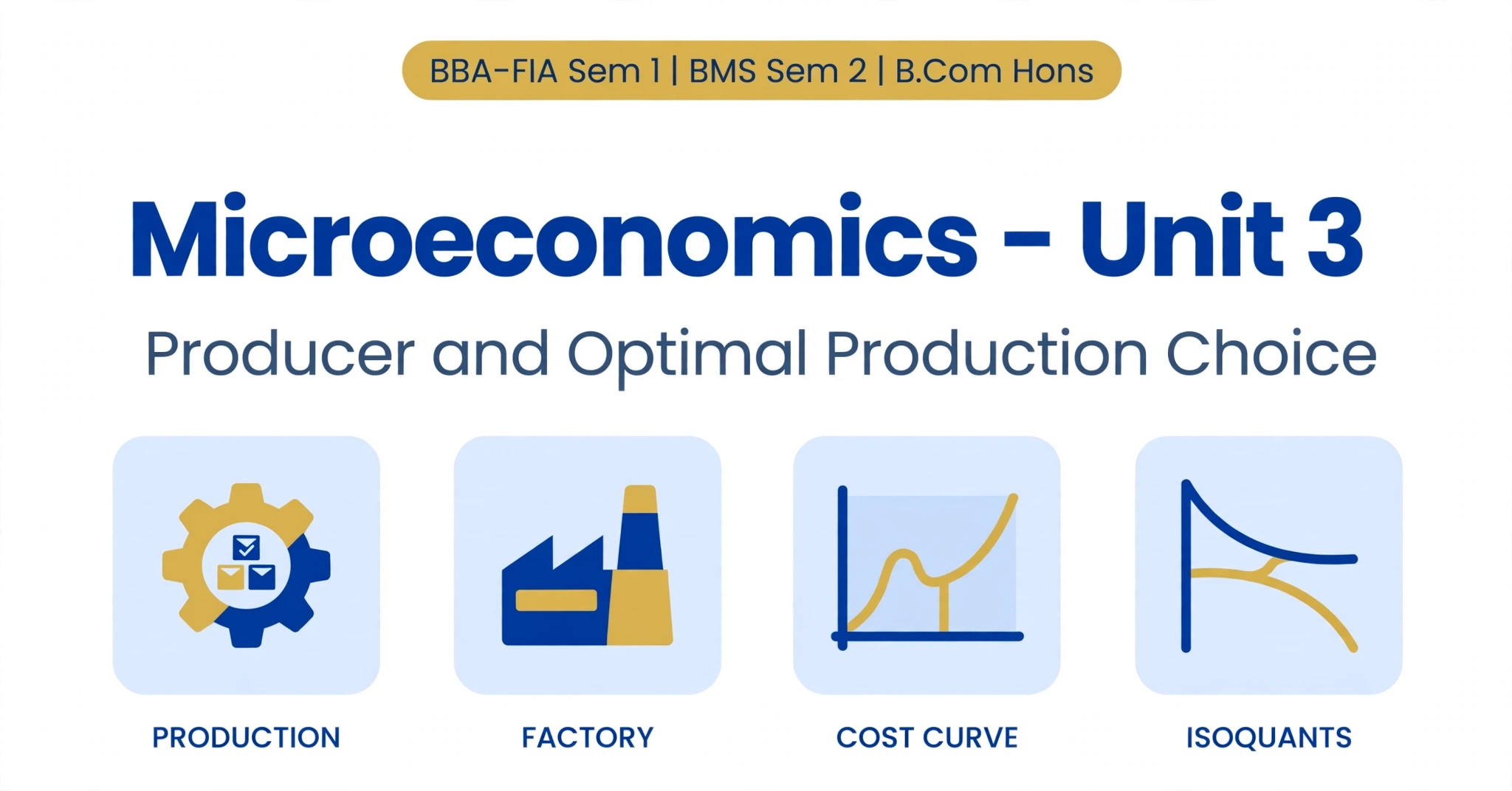
Producer Behavior and Optimal Production Choice—Microeconomics Notes (Unit 3)
Introduction to Production Theory
Production theory explains how firms combine resources such as labor, capital, land, and raw materials to produce goods and services. The main objective of a firm is to produce the desired output at the lowest possible cost by choosing the most efficient combination of inputs.
This unit explains short-run and long-run production, diminishing marginal returns, isoquants, isocost lines, and traditional and modern cost theories.
1. Short-Run Production
In the short run, at least one factor of production remains fixed (usually capital), while other inputs like labor can be varied.
Types of Product
Total Product (TP): Total quantity of output produced using available inputs.
Marginal Product (MP): The extra quantity of output generated when one more unit of a variable resource is employed.
Average Product (AP): Output produced per unit of the variable input.
Formulas:
\[
MP = \frac{\Delta TP}{\Delta L}
\]
\[
AP = \frac{TP}{L}
\]
Where \( L \) = quantity of labor.
2. Law of Diminishing Marginal Productivity
The Law of Diminishing Marginal Returns states that when additional units of a variable input are added to fixed inputs, the marginal product of the variable input will eventually decrease (other things remaining constant).
Example:
In a factory with a fixed number of machines, hiring more workers initially increases production. However, after a certain point, additional workers contribute less extra output because of overcrowding and limited machines.
Relationship between TP, MP, and AP:
Total product increases when marginal product is positive.
Total product starts declining when marginal product becomes negative.
Average Product stops rising and reaches its peak when MP equals AP.
3. Stages of Production
Short-run production is divided into three stages:
Stage I – Increasing Average Product
Average product rises as more units of the variable input are employed. Fixed resources are used more efficiently.
Stage II – Diminishing Marginal Returns
Marginal product decreases but remains positive. Total product continues to increase at a decreasing rate.
This is the economically relevant stage of production.
Stage III – Negative Marginal Returns
Marginal product becomes negative, and total product starts falling. Adding more variable input reduces total output.
4. Long-Run Production and Isoquants
All inputs can be changed in the long run. Firms can change labor, capital, plant size, and technology.
Isoquant
An isoquant is a curve that shows different combinations of two inputs that produce the same level of output.
Properties of Isoquants:
Downward sloping
Convex to the origin
Higher isoquants represent higher output.
Isoquants do not intersect.
5. Isocost Line
An isocost line shows different combinations of two inputs that a firm can purchase with a given total cost.
Equation of Isocost Line:
\[
C = P_L \cdot L + P_K \cdot K
\]
Where:
\( C \) = Total cost
\( P_L \) = Price of labor
\( P_K \) = Price of capital
Slope of the Isocost Line: \( -\frac{P_L}{P_K} \)
6. Optimal Combination of Resources (Producer Equilibrium)
A firm achieves the optimal combination of inputs when it produces a given output at the lowest possible cost.
Condition for Producer Equilibrium:
\[
MRTS_{LK} = \frac{P_L}{P_K}
\]
Or equivalently:
\[
\frac{MP_L}{P_L} = \frac{MP_K}{P_K}
\]
This means the firm is using inputs efficiently so that the additional output obtained per rupee spent on each input is equal.
7. Traditional Theory of Cost
Short-Run Costs
Total Fixed Cost (TFC): Expenditure that does not depend on the quantity produced.
Total Variable Cost (TVC): Expenditure that changes as the firm produces more or fewer units.
Total Cost (TC): \( TC = TFC + TVC \)
Average Cost (AC): \( AC = \frac{TC}{Q} \)
Marginal Cost (MC): \( MC = \frac{\Delta TC}{\Delta Q} \)
Long-Run Costs
In the long run, all inputs are variable.
Long-Run Average Cost (LRAC):
\[
LRAC = \frac{LRTC}{Q}
\]
The LRAC curve is U-shaped and is known as the envelope of short-run average cost curves.
8. Modern Theory of Cost
Economies of Scale:
Long-run average cost falls as the firm increases its scale of production due to specialization, bulk buying, and better technology.
Diseconomies of Scale:
Long-run average cost rises when the firm becomes too large due to managerial inefficiencies and coordination problems.
Learning Curve:
Production costs decline over time as workers and the firm gain experience and improve efficiency.
Conclusion
Unit 3 – Producer Behavior and Optimal Production Choice explains how firms decide production levels and choose the best combination of inputs. Key topics include short-run and long-run production, the law of diminishing returns, isoquants, isocost lines, traditional cost concepts, and modern cost theory. A clear understanding of these concepts is essential for BBA and BMS students preparing for microeconomics examinations.
Frequently Asked Questions (FAQs)
1. What is short-run production?
In the short run, at least one factor of production remains fixed (usually capital), while other inputs such as labor can be varied.
2. What is the Law of Diminishing Marginal Productivity?
It states that when additional units of a variable input are added to fixed inputs, the marginal product of the variable input eventually decreases.
3. What is an isoquant?
An isoquant is a curve that shows different combinations of two inputs (labor and capital) that produce the same level of output.
4. What is an isocost line?
An isocost line shows all combinations of two inputs that a firm can purchase with a given total cost.
5. What is the condition for producer equilibrium?
Producer equilibrium occurs when the Marginal Rate of Technical Substitution (MRTS) equals the ratio of input prices (MRTS = PL / PK).
6. What is the difference between economies and diseconomies of scale?
Economies of scale occur when long-run average cost falls as output increases, while diseconomies of scale occur when long-run average cost rises as the firm becomes too large.